Note: FogVolumes are available in 4.0 alpha 1 and later. This post provides a technical overview for a feature that is already available in the current 4.0 alphas.
On top of the existing non-volumetric fog, Godot 4.0 introduces a new type of fog: Volumetric Fog. For the 4.0 release, we decided to take Volumetric Fog one step further with the addition of FogVolumes. These allow users to dynamically place fog and control complex fog effects with shaders.
This post starts off with a high-level description of what FogVolumes are and how to use them, and then includes some technical details about what is going on under the hood and how we get them to render so fast.
Volumetric fog
Volumetric Fog uses a 3-dimensional buffer to calculate and store fog density values allowing fog to interact with light and shadows in a way that the previous non-volumetric fog never could. Volumetric Fog adds a new dimension of realism to 3D scenes.
For example, here is a view of Crytek’s popular Sponza scene (well, popular among graphics developers).
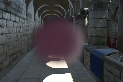
Turning on Volumetric Fog, we can instantly make it a little more interesting!
As you can see, Volumetric Fog responds to both light and shadow automatically. It also updates in real time!
By default, Volumetric Fog covers the entire scene with a uniform density, but sometimes specific effects call for having fog in only one portion of a scene (like in the above video). For that, you need FogVolumes.
FogVolume nodes
FogVolumes come in many different shapes, they can either be boxes, ellipsoids, cones, cylinders, or they can cover the whole world. Naturally, it is more efficient to use a box, ellipsoid, cone, or cylinder shape as they limit the region over which the fog is calculated.
By default, FogVolumes add fog into the scene. The fog model we use internally is based on density, albedo, and emission which are all additive properties. This means that when FogVolumes overlap, we need only add the density, albedo, and emission from the respective FogVolumes and the results will look correct.
The same goes for subtraction. You can use a negative density to subtract one volume from another to create more complex shapes if you need to, or if you need to keep fog from accumulating somewhere like in a house or other building.
FogVolumes are 3D nodes that can be placed in the scene like other nodes and they immediately react to the existing lighting conditions and other objects in the scene. The only restriction is that Volumetric Fog must be enabled in the Environment for the FogVolumes to be visible.
If you wish to disable global volumetric fog but still want to have volumetric fog constrained within specific areas, enable Volumetric Fog and decrease its density to 0.0.
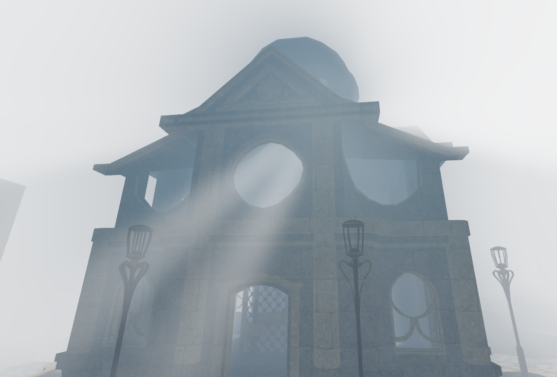
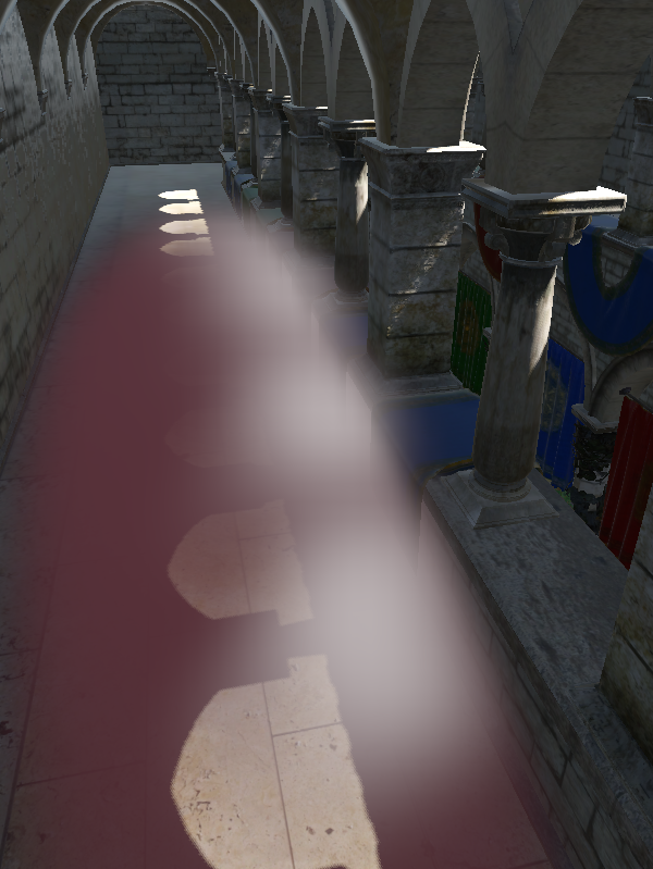
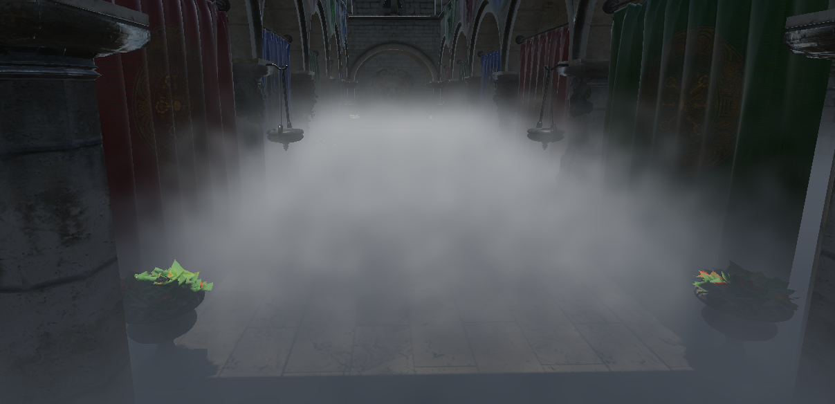
Pictured below is a FogVolume partially intersecting a light beam. As you can see, the beam of light penetrates through the volume in a plausible way.
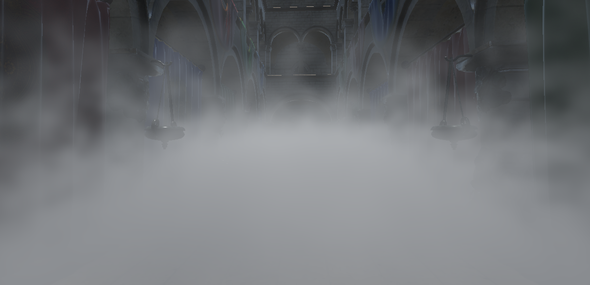
If you crank up the detail (not recommended for performance reasons), you can acheive very sharp-looking light shafts in a constrained area. You can also choose to decrease the maximum volumetric fog rendering distance to improve volumetric fog detail without incurring a performance cost.
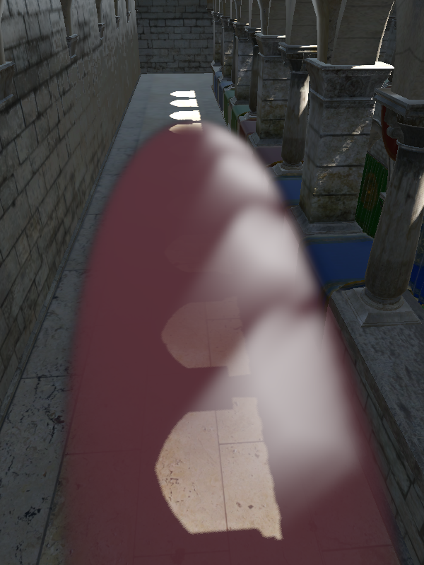
At the default settings, the light still looks plausible, but not nearly as detailed. On the bright side, at default settings, Volumetric Fog and FogVolumes are efficient even on integrated GPUs.
FogVolumes come with a built-in FogMaterial which allows users to quickly and easily set basic properties like, albedo (color), density, emission, and height falloff.
Perhaps the most exciting part about FogVolumes is the introduction of the fog shader type. FogVolumes can be controlled with custom Fog shaders to add detail or to shape them however you want. For example, you can vary fog density according to an animated noise pattern.
FogVolumes respond to lighting in real time, the exact same way that Volumetric Fog does.
Technical details
When starting to work on FogVolumes, we wanted to ensure that users could be creative with them without running into performance barriers. In particular, we wanted users to be able to have a large number of FogVolumes present in the scene without incurring a large performance penalty. Similarly, we wanted to allow users to combine and overlap FogVolumes without restriction.
Volumetric Fog uses an optimized algorithm to calculate fog based on the approach described by Bart Wronski in his 2014 SIGGRAPH presentation “Volumetric Fog: Unified Compute Shader-Based Solution To Atmospheric Scattering”.
The Wronski approach to volumetric scattering is widely used by many engines, so we won’t go into depth into it. The important thing to take away is that we calculate the volumetric lighting in a large 3-dimensional buffer called a “froxel buffer”. Froxels are frustum-aligned voxels. Another way to think about it is grid-aligned and scaled with the camera’s frustum. Therefore, cells close to the camera are quite small and the cells grow larger as they get further from the camera due to perspective projection. By default, we use a 64×64×64 froxel buffer, but this can be adjusted in the Project Settings. What makes the approach so fast is that you only calculate lighting for the cells in the froxel buffer and then, when drawing meshes, you only need to look up the fog value from the froxel buffer.
To make rendering FogVolumes efficient, we render them to the froxel buffer used for Volumetric Fog instead of rendering each volume independently.
This allows us to detach light rendering from FogVolume rendering and support huge numbers of lights, independent from the number of FogVolumes.
In doing so, we run into a small problem: accessing the same piece of memory on the GPU can result in problems with rendering. To resolve those problems, each rendering command needs to wait for the one before it to complete and you end up in a situation where your GPU spends most of its time waiting for more work instead of actually doing work. For only a few volumes that are spread apart, this isn’t a problem. However, we want to be able to support scenes with hundreds of volumes or more!
Let’s take a step back to understand why it can be a problem to render multiple volumes at the same time by looking at a single froxel in the buffer.
density = 0
The density starts at 0.
// First, we draw a single primitive with a density of 1.
density += 1

// What the code is really doing is essentially:
temp = density
density = temp + 1  // Density is now 1.
To add to density, we actually need to do three operations:
- copy the value of density,
- add 1 to our local copy of density, and
- write back that data to density.
Let’s look at what can happen if two volumes try to draw at the same time.
temp1 = density
temp2 = density  // Uh oh.
density = temp1 + 1  // Density is 1.
density = temp2 + 1  // Density is still 1.
What went wrong here is that one GPU operation overwrote the result of the other. In the end, the density of that cell ends up being half of what it should be. To the end user, this would look like a chunk of the scene with missing fog.
We clearly need to do something to avoid this issue. One approach that many engines adopt is to render volumes using geometry shaders to generate and render slices. This works well because each “slice” of the volume can be rendered independently with “additive” blending directly into the target froxel buffer. Using additive blending in a fragment shader allows the GPU to draw the fog slices in a way where it doesn’t matter in what order they are drawn. This allows the GPU to draw everything as fast as it can without waiting on other rendering operations.
We wanted to avoid using geometry shaders as they are poorly supported on a lot of hardware, especially integrated graphics and mobile. Instead, we went with a different solution based on compute shaders. To avoid stalling the GPU between draw calls, we use atomic operations in the shader. Atomic operations are special versions of common operations (add, or, min, max) that can operate on the same memory without running into the problem described above. In our case, this allows the GPU to draw multiple volumes at the same time, and doesn’t risk the volumes overwriting each other.
In order to take advantage of atomic operations, we needed to make many changes to how we store the fog information. In particular, GLSL only supports atomic operations on integers. The values we are working with (density, albedo, emission) are all floating-point (and albedo and emission each contain 3 channels!). The first step was to encode the floating-point values into integers in a way where they could still be additively blended. In the end, we settled on using 3 textures the size of the froxel buffer each with a single 32 bit unsigned integer per cell.
- Density is encoded as a signed 32-bit integer by multipling the floating-point density by 1024. This allows a range of -64 to 64 for density. In particular, the negative range is necessary to allow for subtracting volumes.
- Albedo is encoded as a “scattering” which is to say that it is multiplied by density and clamped to the 0 to 1 range before being stored. Then, it’s packed into 32 bits as follows:
uint(red * 2047.0) << 21 | uint(green * 2047.0) << 10 | uint(blue * 1023.0);. This gives red and green twice as much precision as blue as they receive 11 bits each, while blue only receives 10 bits. Blue is the least visible color to the human eye, so red and green were chosen to receive higher precision. - Emission is encoded similarly to Albedo. We multiply it with density, but then we clamp to the 0 to 4 range. This way, emission is able to add a little bit of dynamic range. 4 was chosen as a reasonable range to allow some dynamic range but maintain some precision. The exact range can be adjusted at a later date based on user feedback.
We use such simple linear scaling of values so that the fog properties can be simply added together in their unsigned integer format. If we used a non-linear encoding of values, we wouldn’t be able to add them together without running into other artifacts.
Using such a simple approach creates another interesting problem: individual color channels can overflow and bleed into their neighbors. A little bit of color bleeding is acceptable as it only impacts the least signfificant bit (for Albedo it would add 1 / 2043, for Emission it would add 1 / 512), but a color overflowing is a huge problem.
Let’s look at an example. Suppose one cell’s blue albedo channel reached 1.0 (in binary: 11 1111 1111), and then suppose another FogVolume overlaps that cell with a blue value of at least 0.00097 (in binary: 00 0000 0001) after adding them, 1 bit will be added to green and blue will turn to 0.0 (in binary: 00 0000 0000). This is, of course, a huge problem for us.
The solution we settled on rests on one key behaviour of GLSL’s atomicAdd() function. When adding a given value to value stored in memory, atomicAdd() is guaranteed to return the value of the memory immediated before the addition. Accordingly, we can replay the addition locally and check if any color channel overflows. If it does, we take the atomicOr() of that color channel with the same number of bits set to 1 to force it to its maximum value (1 in the case of Albedo, or 4 in the case of emission). Of course, the atomicOr() is only necessary when we detect an overflow.
In practice, here’s how that might look:
// Albedo from the current Fog Volume.
new_albedo = 0000 0000 000 0 0000 0010 00 00 1000 0101  // R = 0.0, G = 0.0039, B = 0.13

// `current_albedo` is returned by our call to `atomicAdd()`.
current_albedo = 0011 1111 010 1 1111 1110 00 01 0011 1010  // R = 0.247; G = 0.9966; B = 0.307

// Manually adding `new_albedo` to `current_albedo` in the shader (not using `atomicAdd()`).
local_add = 0011 1111 011 0 000 0000 00 01 1011 1111  // R = 0.248; G = 0.0; B = 0.437

// We detect that green is now lower than it was before; that's not supposed to happen.
// So we create an overflow factor.
overflow_factor = 0000 0000 000 1 1111 1111 11 00 0000 0000  // R = 0.0; G = 1.0; B = 0.0

// We then call `atomicOr()` with the albedo and overflow factor to obtain a final result.
final_albedo = 0011 1111 011 1 111 1111 11 01 1011 1111  // R = 0.248; G = 1.0; B = 0.437
While the results aren’t perfect (we added too much red), the results are close enough and we are able to do this validation very quickly. On top of that, this avoids any memory synchronization issues as all the writes to albedo are done with atomic operations. There’s a gap between the two atomic calls where other atomicAdd()s may modify the memory, but since we’re essentially clamping the value with the overflow factor, we can trust that the other atomicAdd()s won’t hurt anything.
An alternative solution we explored (which was suggested to me by my brother while on a camping trip) was to add a padding bit between each color channel. In binary, our Albedo then looked like RRRR RRRR RRPG GGGG GGGG GPBB BBBB BBBB. This allowed us to avoid the problem of the single bit bleeding, as we could use an atomicAdd() to clear the padding bits, but it still required us to “replay” the addition to avoid the rest of the impact of the overflow. In the end, we decided keeping the extra bit of precision in the red and green channels was preferable to protecting ourselves against the overflow.
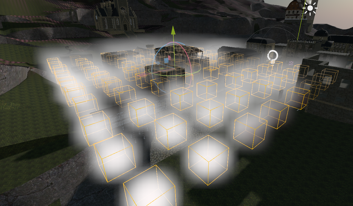
Below is one of the test scenes I used while stress testing FogVolumes. It contains 96 simple volumes which each inject a little bit of density and color into a small area.
Now for the interesting part. Below is a screen capture of a page from AMD Radeon GPU Profiler showing a zoomed in section of the rendering frame. The top bars represent how much work the GPU is doing and the bottom bars show individual commands that have been sent to the GPU and how long they take.
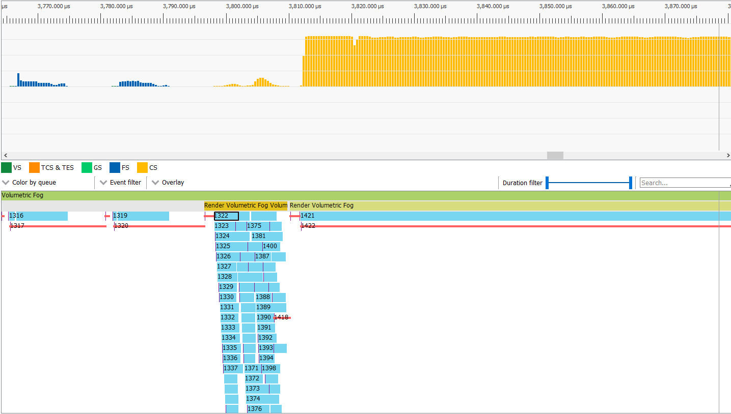
As you can see, the FogVolumes are mostly rendered at the same time, and even then, they can’t saturate the GPU – of course this changes when using larger or more complex fog shaders. To the right, you can see that the lighting calculations are able to saturate the GPU and keep it busy.
Overall, we’re quite happy with the results and are confident that users will be too.
That was just the tip of the iceberg. In adding FogVolumes, we overcame a few interesting technical challenges and faced a number of tradeoffs in designing a system we hope is fast, flexible, and friendly for users. For more details about the implementation, please see the pull request on Github.
Support
Godot is a non-profit, open source game engine developed by hundreds of contributors on their free time, and a handful of part or full-time developers, hired thanks to donations from the Godot community. A big thankyou to everyone who has contributed their time or financial support to the project!
If you’d like to support the project financially and help us secure our future hires, you can do so on Patreon or PayPal.